

Time Series Metrics, Sampling Theory, and Enterprise Monitoring
I have played musical instruments since I was young, and in the 1990s I got heavily into recording. My parents kindly bought me a Yamaha 4-track cassette recorder and Music-X on the Amiga, and I spent a lot of time recording guitar and bass tracks, plus drums and keyboard programmed using Music-X.
While at the university where I was studying mechanical engineering, I hang around with people from the audio engineering course so I can get in the recording studios with them, tinkering with the Neve desk with 24-track Soundcraft 2-inch real-to-reel. During this time these friends introduced me to the book John Watkinson’s The Art of Digital Audio explained the thery of sampling, quantization, dynamic range, filtering, and I was absolutely facinated. Separately within my mechanical engineering course, one of the lecturers introduced me to the book Numerical Recipes in C and I was able to articulate some of the audio theories in code, like learning about Fast Fourier Transform and implementing algorithmic equalisation etc. It made me think much more carefully about how data is captured, processed, stored, transformed, approximated, and compressed and so on.
When I came into the enterprise wold and looking at monitoring, I could not help thinking about the sampling theory and attempted to discuss this with my colleagues but they were simply not interested. We can use modern words like observability, dashboards, retention, rollups, and cardinality, but the underlying question is still very simple: how often did we sample the system, and how much of the original behaviour can we still see in the data?
That is why coarse monitoring has never sat well with me. If you sample too in-frequently, the graph stops being a faithful record of what the system did and becomes a simplified summary of it.
Does the sampling theory apply to enterprise monitoring?
Yes, in my humble opinion, it does. In plain terms, the theorem says this: if you want sampled data to represent the original signal correctly, you need to sample fast enough for the fastest behavior you care about. If you do not, fast behavior gets distorted and can appear as slower behavior that did not actually happen. In monitoring, that means short latency spikes, queue bursts, and short GC pauses can be hidden or misrepresented when collection intervals are too coarse.
The equations are still useful because they make that limit explicit.
Sampling period:      T_s = 1 / f_s
Nyquist frequency:    f_N = f_s / 2
Nyquist condition:    f_s >= 2 f_max
PCM dynamic range:    DR ≈ 6.02 N + 1.76 dB
f_s is the sampling frequency and T_s is the interval between samples. f_N is the Nyquist frequency, which is half the sample rate. Any frequency content above f_N will fold back into the baseband after sampling unless it is removed before sampling.
That fold-back is aliasing. A useful way to think about it is:
f_alias = |f_signal - k f_s|where k is the integer that maps the result into [0, f_s/2].
Example: if f_s = 40 Hz and a component exists at f_signal = 30 Hz, then it aliases to 10 Hz in sampled data. The sampled signal now contains energy that was never actually present at 10 Hz in the source. That is why Nyquist is not only about sample rate. It is also about pre-sampling filtering.
In audio, that filtering is anti-alias filtering in the A/D path and reconstruction filtering in the D/A path. In monitoring, there is usually no explicit anti-alias filter. The equivalent control is the collection interval plus any pre-aggregation in exporters, agents, or query windows. If the interval is too coarse, short events are effectively folded or averaged into slower-looking behaviour.
There is another important caveat. The classic theorem assumes a band-limited signal. Enterprise systems are usually not band-limited in a strict sense because they contain bursts, steps, queue transitions, retransmits, GC pauses, and other non-periodic events. In practice, that means the theorem still gives useful intuition, but real systems require faster sampling than a clean sinusoidal model would suggest if the goal is reliable diagnosis.
What sampling rate means in audio and in monitoring
In digital audio the relationship between source and sample rate is easy to understand. A 44.1 kHz system gives you a sample every 22.68 microseconds and a 48 kHz system gets that down to 20.83 microseconds. Those rates are used because transients are fast, harmonic content is dense, and our ears notice when the digital version is not keeping up with the original signal.
Enterprise monitoring often acts as if those constraints do not apply once the signal comes from software instead of from a microphone. Many platforms still rely on 60-second resolution for custom metrics, or they collect faster for a short period and then retain at a coarser rate once the data gets older. That may be acceptable for long-range trend reporting, but it is weak for incident diagnosis.
The contrast is easier to see when it is laid out directly.
| Concept | Digital audio | Enterprise metrics |
|---|---|---|
| Sampling rate | 44.1 kHz, 48 kHz, 96 kHz and higher | Commonly 60 s, 30 s, 15 s, or 5 s |
| What is being preserved | Waveform shape over time | Operational behavior over time |
| Failure when undersampled | Aliasing, smeared transients, false tones | Missing spikes, flattened bursts, misleading averages |
| Dynamic range concern | Noise floor to clipping | Quiet baseline to short-lived pathological spikes |
| Reconstruction goal | Faithful playback | Faithful diagnosis and alerting |
There is also a simple way to think about how often fast incidents disappear. If an event lasts tau seconds and the sample interval is T_s, then for a simple pulse that is not averaged across the bucket the probability of missing it entirely is roughly:
P(miss) ≈ 1 - (tau / T_s), when tau < T_sSo a 10-second event sampled every 60 seconds has a strong chance of vanishing altogether if the sample phase happens to be unhelpful.
Why Sony and Philips landed on 44.1 kHz and 16-bit
As with all audio medium, CD’s have somewhat become the legacy system, but it was a revolutionary system when it first came out. Sony and Philips jointly developed the digital audio format and and how the data is imprinted and read from a tiny disk. They considered many aspects including the quality of the audio, and the duration of music that could be fit on one disc. Sony’s requirement was to be able to fit Beethoven’s 9th Symphony which is 74 minutes and that is what they delivered.
The first requirement was the human hearing range. Human hearing range is typically quoted up to about 20 kHz in young listeners, so Nyquist says the sample rate must be above 40 kHz. A 44.1 kHz rate gave 22.05 kHz Nyquist and left enough transition band for real anti-alias and reconstruction filters in the hardware available at the time.
The second constraint was dynamic range. With the common approximation DR ~= 6.02N + 1.76, a 16-bit system gives about 98 dB theoretical range, with about 96 dB commonly used as the practical headline. That was enough to beat cassette noise by a wide margin and support serious listening in home and studio contexts.
The third constraint was data volume and channel coding overhead. Stereo PCM at CD format is:
Bit rate = 44,100 samples/s * 16 bits/sample * 2 channels
         = 1,411,200 bits/s
         = 176,400 bytes/s
         ~= 10.1 MB/min
At 74 minutes, that is about 783 MB of raw PCM audio. On top of that, the format adds framing, subcode, CIRC parity, and EFM channel coding, so the physical on-disc channel representation is far larger than the raw audio stream and comfortably above 1 GB. That overhead is exactly what made the medium resilient to scratches and burst errors.
There was also a manufacturing and ecosystem angle. Early digital audio mastering pipelines used video-based PCM adaptors, and 44.1 kHz mapped cleanly enough to both NTSC and PAL workflows. So the final number was not only about hearing and math. It also fit the production chain Sony and Philips could ship at scale.
What our requirements were
The same way CD had explicit design targets, we needed explicit targets for enterprise monitoring.
- We needed high temporal resolution so short incidents are visible, which is why we treated 5-second collection as a baseline rather than an optional mode.
- We needed broad coverage across system, JVM, coordinator, table, and threadpool layers because latency diagnosis fails when one of those layers is missing.
- We needed low collection overhead on Cassandra nodes, so collecting more detail would not become the cause of new performance problems.
- We needed practical retention and downsampling, so long-term views stay affordable while preserving the shape of important events.
- We needed operational context with the metrics, including logs, alert routing, and configuration state, so engineers could move from detection to root cause without switching tools repeatedly.
Resolution and dynamic range are different things
One of the oldest confusions in audio is the habit of blending sample rate and bit depth into one vague idea of quality, even though they are not the same thing at all. Sample rate tells you how finely time is being represented, while bit depth tells you how finely amplitude is being represented and what theoretical dynamic range the system can support.
The enterprise analogy is not exact because most monitoring platforms already have enough numeric precision for ordinary metric values, so in practice the real bottleneck is usually temporal resolution followed by what I would call semantic resolution. Are you only capturing coarse host metrics, or are you also seeing GC behavior, disk wait, queue build-up, table-level latency, and threadpool pressure? A one-minute signal is already compromised, and a one-minute signal at the wrong layer is barely diagnostic at all.
| Dimension | In audio | In enterprise monitoring |
|---|---|---|
| Temporal resolution | Sample interval in microseconds | Scrape or collection interval in seconds |
| Amplitude resolution | Quantization step from bit depth | Usually not the limiting factor |
| Dynamic range | Distance between noise floor and clipping | Ability to preserve both ordinary behavior and short severe excursions |
| Semantic resolution | Channels, mix, microphone placement | Host, JVM, process, queue, table, percentile, label dimensions |
That final row is where the monitoring problem becomes especially painful. If you never captured the interesting layer of the system in the first place, no clever storage engine will restore it later.
A short monitoring example
Below is an example chart that looks very different once the sample interval changes. At 5-second resolution the spike is obvious. By 30 seconds it already looks more like a broad shelf, and by 60 seconds an engineer could easily underestimate how abrupt the original event really was.
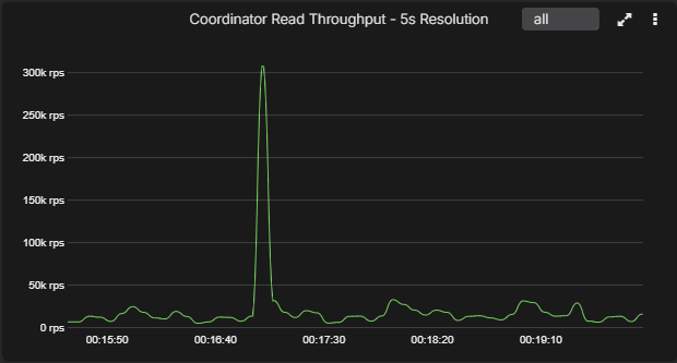
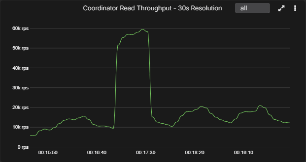
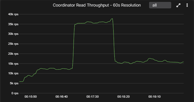
That is not just a difference in how the graph looks, because it changes the whole investigation. A sharp transient suggests one class of problem, while a broad one-minute plateau suggests another. One points you toward bursty load, queue thresholds, fast infrastructure events, or GC interruption. The other points you toward something slower and more sustained.
For databases this gets more serious because so many damaging behaviors are brief and expensive at the same time. A read path can suddenly touch too many SSTables, a queue can back up for fifteen seconds and then drain, a tombstone-heavy workload can flare and disappear again, a network fault can come and go between coarse samples, and a JVM pause can be obvious to clients while being barely visible in a low-resolution monitoring system.
Why enterprise metrics are usually sampled at low resolution
In many enterprises the metrics are sampled at 30s intervals or at 60s.
The reason for this is predominantly the cost. The longer answer is that platforms often optimize for their own economics before they optimize for your ability to reconstruct an incident cleanly.
Higher-frequency collection increases storage, network traffic, label pressure, and collection overhead, and in some systems that overhead lands directly on the monitored process. Cassandra over JMX is one obvious example, because if you collect too much, too often, through an expensive interface, you can end up making the act of observation part of the operational problem.
Even so, there is a stubborn fact sitting underneath all of this. In many enterprise stacks the sample interval is chosen around the comfort of the observability product rather than around the shape of the workload, and I have always found that backwards because if the point of monitoring is to understand what the system did, then the system should set the bar and the tooling should work to meet it.
Compression, retention, and the value of old data
Time-series systems do not merely collect; they also compress, roll up, and eventually discard. That sounds harsh, but it is exactly what they should do if they are designed properly. The real question is what to throw away and when.
| Class | Examples | What it does |
|---|---|---|
| Lossless compression | Delta encoding, delta-of-delta, XOR compression, run-length encoding | Stores the same series more efficiently without changing its meaning |
| Lossy summarization | Bucket averages, min/max rollups, LTTB, reservoir-style reductions | Keeps a simplified representation that is cheaper to retain or display |
The Gorilla paper remains one of the better examples on the lossless side because it takes advantage of two properties that show up repeatedly in time-series workloads: timestamps are regular or nearly regular, and adjacent values tend to be strongly correlated. That makes delta-of-delta encoding a natural fit for time and XOR-based encoding a very effective fit for values.
Other engines use variations on the same idea. Delta encoding is common because change between neighboring samples is often small, run-length encoding works well when states repeat, and some systems add block or dictionary compression once query patterns become more archival than interactive.
Monitoring introduces one more idea that people should be more willing to say out loud, which is that old data is usually worth less than recent data. It is not worthless, but it is worth less. When an incident is live, raw high-resolution samples are precious. Six months later, what you usually need is not sample-perfect reconstruction but the trend, the shape, the turning points, and the context that explains whether the system changed regime over time. That is why downsampling makes sense, provided you preserve the structural character of the original series.
Downsampling method
Plain averages are often destructive because if a bucket contains one violent spike and fifty seconds of calm, the average mostly preserves the calm and hides the event you actually cared about. Min and max rollups are an improvement, but they still do not preserve the shape well enough when you need to render long spans without losing the visual turning points.
That is why AxonOps adopted Largest-Triangle-Three-Buckets for downsampled visualization while retaining raw collection at 5-second intervals.
LTTB works in four steps:
- Keep the first and last points.
- Split the remaining points into equal-size buckets.
- For each bucket, compute the average point of the next bucket.
- Select the point in the current bucket that forms the largest triangle with: the previously selected point and the next-bucket average point.
The triangle area used by LTTB is:
Area = |x_a(y_b - y_c) + x_b(y_c - y_a) + x_c(y_a - y_b)| / 2The algorithm picks point b that maximizes this area for each bucket. In practice this keeps turning points and spikes that would disappear with simple averages.
For monitoring this is a good fit because engineers mostly use downsampled charts for overview and navigation. They zoom in for detail. LTTB keeps overview charts readable while preserving where the signal changed direction or jumped.
It is also important to be clear about what LTTB is not. It is a visualization downsampling method. It is not a replacement for raw samples in alerting, SLO calculations, or incident forensics. In AxonOps, the alerts and root-cause workflows still run on high-resolution raw data.
That is the compromise that works: raw high-frequency data for detection and analysis, with LTTB downsampling for efficient long-range visualization.
Why AxonOps samples at 5 seconds
The raw collection interval in AxonOps is every 5 seconds. That is much higher than a great deal of enterprise custom-metric collection, and it was not chosen by accident.
Five seconds is nowhere near audio-rate sampling, but that is not the relevant comparison. The important point is that many operational problems in distributed systems unfold across a span of a few seconds to a few tens of seconds. Once you sample at one-minute intervals, you are no longer looking at the event itself but at a simplified version of it.
That is also why richer metric coverage matters so much. High-resolution host metrics help, but high-resolution database metrics are where diagnosis becomes much more convincing. When you can put CPU, I/O wait, GC pause behavior, queue build-up, coordinator percentiles, and table-level signals side by side, you are no longer staring at a generic health graph and trying to invent meaning from it.
More than anything else, that is what stayed with me from the digital-audio years: if the representation is poor, you stop seeing what really happened and start seeing a rough approximation of it. I could not bear listening to digitally encoded music that is anything less than 44.1KHz and 16-bit. Having been working with the AxonOps monitoring platform at 5-seconds resolution, it’s a major frustrations when seeing anything less!
If you got here then you’re probably care about your infrastructure and monitoring. If you’ve always felt monitoring Kafka or Cassandra in general have been substandard, come and try AxonOps, and plug your existing clusters. You should be able to do this within minutes and see the amazing set of dashboards with high resolution metrics showing you the insights you’ve never seen before on your clusters.
References
The theory and algorithms behind this post are worth reading directly.
- Harry Nyquist, Certain Topics in Telegraph Transmission Theory, Bell System Technical Journal, 1928.
- Claude E. Shannon, Communication in the Presence of Noise, Proceedings of the IRE, 1949.
- Sveinn Steinarsson, Downsampling Time Series for Visual Representation, University of Iceland, 2013.
- Tuomas Pelkonen et al., Gorilla: A Fast, Scalable, In-Memory Time Series Database, PVLDB, 2015.
If you want to see the monitoring side of this discussion applied to Cassandra in more depth, the follow-on reads are Monitoring Cassandra: The Cost of Collecting Metrics and Cassandra Monitoring Tools Comparison 2026.